Rotational Resonance
Problem
Create a z-matrix for an alanine molecule using some reasonable assumptions about its geometry.
Neglect the chemical shifts and CSA’s on protons and use the following 13C chemical shift parameters. Isotropic chemical shifts (ppm): 176.8 (CO), 50.9 (CA), 19.8 (CB). Chemical shift anisotropy (ppm): -71 (CO), -20 (CA) -12 (CB). Chemical shift asymmetry: 0.84 (CO), 0.44 (CA), 0.76 (CB). CSA orientation for the CO carbon: the most shielded direction is perpendicular to the sp2 plane; the least shielded direction is along the CO-CA bond. CSA orientation for the CA carbon: the most shielded direction is perpendicular to the H-CA-CB plane; the least shielded direction is 20º away from the H-CA bond towards the CA-CB bond. CSA orientation for the CB carbon: the most shielded direction is parallel to the CA-CB bond; the least shielded direction can be chosen as you please. Hint,: the most shielded direction coincides with the z principal component axis in all three CSA tensors above.
Compute the R2 (rotational resonance) polarization exchange curves between CO and CA in a [CO,CA]-labeled sample and between CO and CB in a [CO,CB]-labeled sample for n=1 resonance (spinning frequency coincides with the chemical shift difference). Sample one point per rotor period. Start with the initial density matrix I1z – I2z. Assume a 500 MHz spectrometer. Use a 80 kHz CW 1H decoupling field during the R2 exchange. Perform these calculations for the following spin systems.
First, do this in the C2 spin systems (without protons). Then add the protons and simulate three different regimes: the CH3 and NH3 groups are hopping infinitely fast (“hot”); only the CH3 groups are hopping infinitely fast (“cold”); no dynamics (“frozen”).
Repeat the simulations with the powder averaging sets of different sizes. Choose a size appropriate for these simulations.
Plot the results of the simulations with protons using the corresponding C2 results as reference (option -ref).
Solution
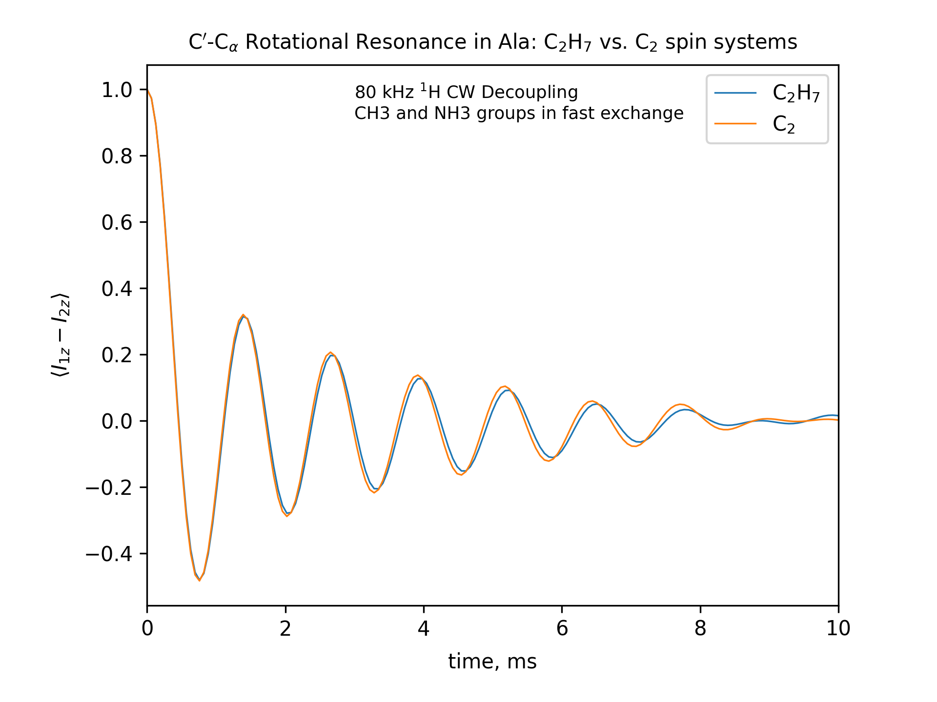
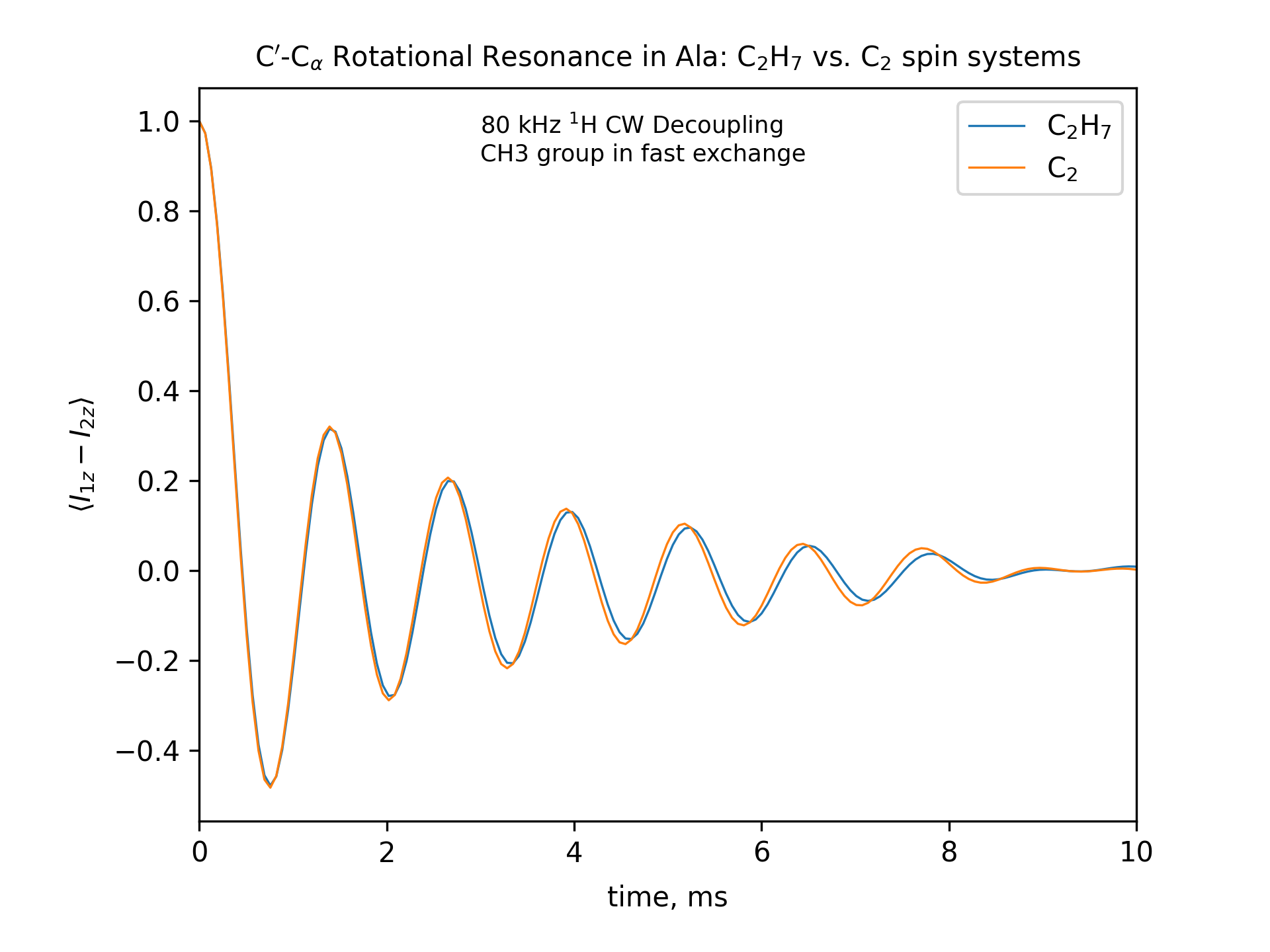
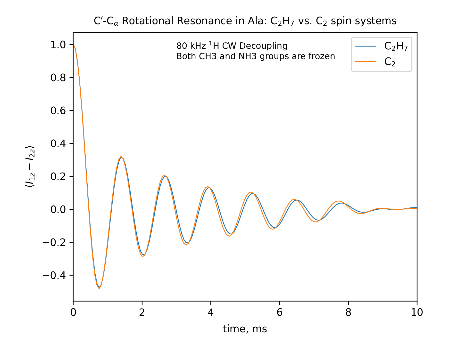
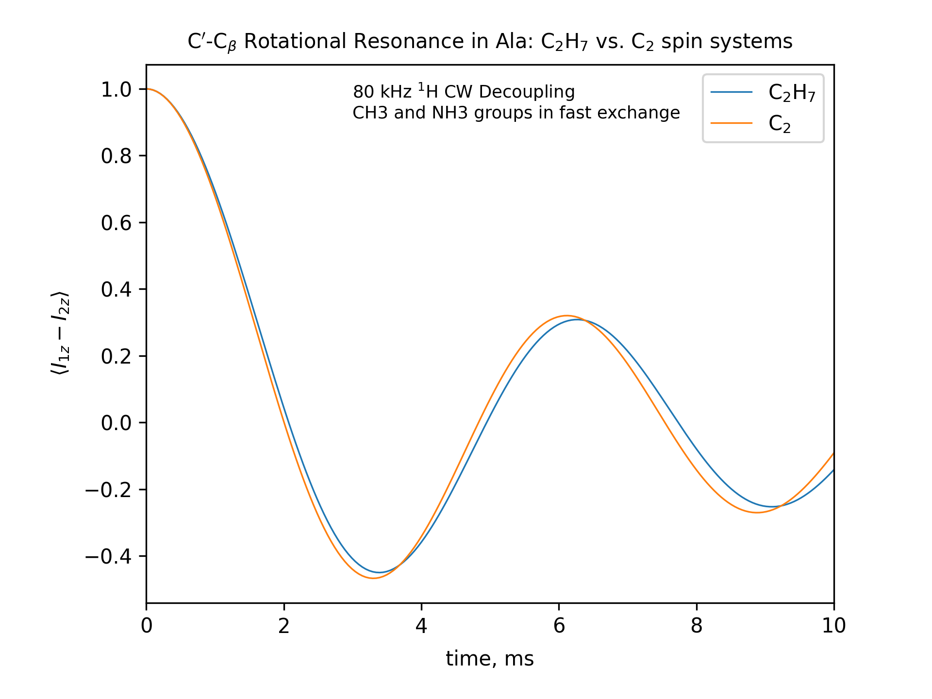
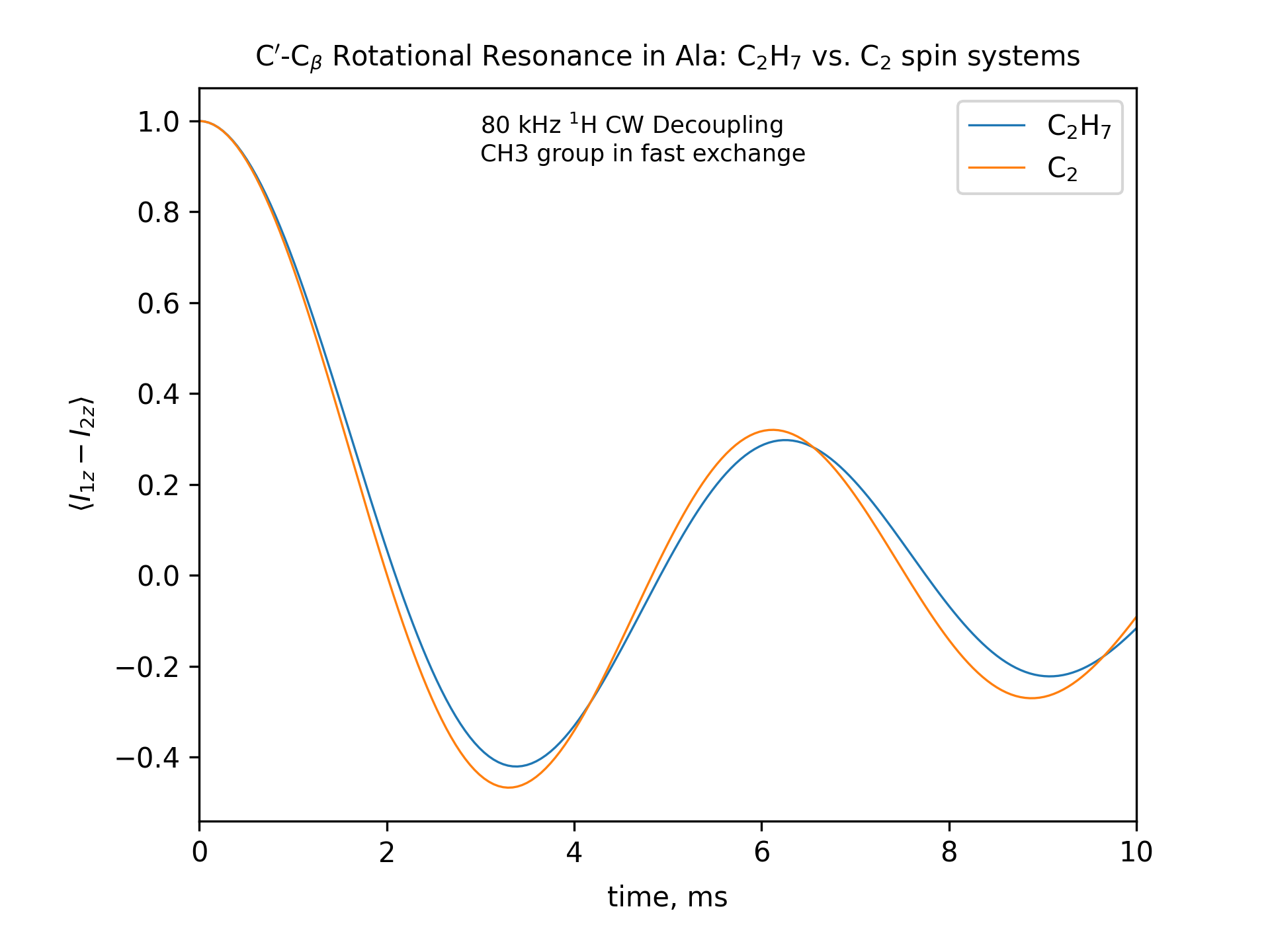
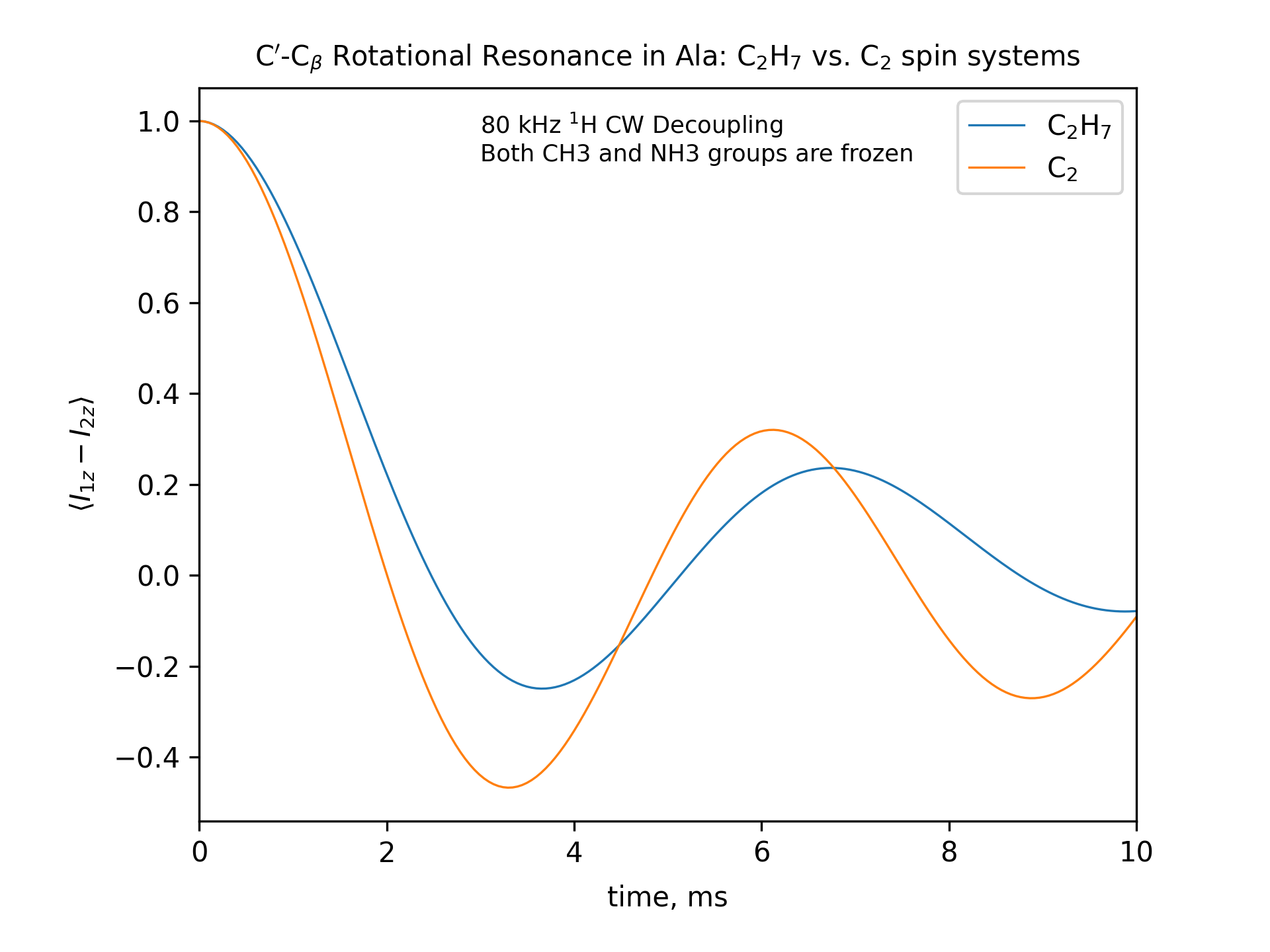
r2-C2
****** The System *******************************************************
spectrometer(MHz)  500
spinning_freq(kHz) 10
channels           C13
nuclei             C13 C13
atomic_coords      *
cs_isotropic       176.8 50.9 19.8 0 0 0 0 0 0 0 ppm
csa_parameters     1 -71  0.84   0   0  0 ppm 1
csa_parameters     2 -20  0.44 -20   0  0 ppm 2
csa_parameters     3 -12  0.76   0 -90  0 ppm 3
j_coupling         *
quadrupole         *
dip_switchboard    *
csa_switchboard    *
exchange_nuclei    *
bond_len_nuclei    *
bond_ang_nuclei    *
tors_ang_nuclei    *
groups_nuclei      (2 1 4) (7 2 3) (2 3 8)
******* Pulse Sequence ***************************************************
CHN 1
timing(usec)     (100)512
power(kHz)         0
phase(deg)         0
freq_offs(kHz)     0
******* Variables *********************************************************

sys2ext_map=["1 X"]
spinning_freq=cs_iso_X-cs_iso_1
freq_1_1_1=(cs_iso_X+cs_iso_1)/2
pulse_1_1_1=1000/spinning_freq

** Figure setup ***********************************************************
q = (X==2)? "alpha" : "beta"
fig_title=f"C$'$-C$_\[q]$ Rotational Resonance in Ala: C$_2$ spin system"
y_label="${\langle}I_{1z}-I_{2z}{\rangle}$"
x_lim=["0 10"]

******* Options ************************************************************
rho0               0.5*I1z-0.5*I2z
observables        I1z-I2z
EulerAngles        rep700
n_gamma            12
line_broaden(Hz)   *
zerofill           *
FFT_dimensions     *
options            -zxmatala.zxmat -re -nr2-C1CX -py
*****************************************************************************
-- Either -macroX=2 or -macroX=3 must be specified at the command line
-- The spinning frequencies used for X=2 and X=3 cases are different. So the total observation times (512 points) will also different. To plot the output results on the same scale, we simply set the same x-axis limits for both cases.
-- CO-CA  oscillations after ~10ms are due to incomplete powder averaging. They can be seen if one uses a higher upper limit in x_lim, e.g., x_lim=["0 21"]
r2-C2H7-hot
****** The System *******************************************************
spectrometer(MHz)  500
spinning_freq(kHz) 10
channels           C13 H1
nuclei             *
atomic_coords      *
cs_isotropic       176.8 50.9 19.8 0 0 0 0 0 0 0 ppm
csa_parameters     1 -71  0.84   0   0  0 ppm 1
csa_parameters     2 -20  0.44 -20   0  0 ppm 2
csa_parameters     3 -12  0.76   0 -90  0 ppm 3
j_coupling         *
quadrupole         *
dip_switchboard    *
csa_switchboard    *
exchange_nuclei    (8 9 10) (11 12 13)
bond_len_nuclei    *
bond_ang_nuclei    *
tors_ang_nuclei    *
groups_nuclei      (2 1 4) (7 2 3) (2 3 8)
******* Pulse Sequence ***************************************************
CHN 1
timing(usec)     (100)512
power(kHz)         0
phase(deg)         0
freq_offs(kHz)     0
CHN 2
timing(usec)      100
power(kHz)         80
phase(deg)         0
freq_offs(kHz)     0
******* Variables *********************************************************

sys2ext_map=["1 X 7 8 9 10 11 12 13"]
spinning_freq=cs_iso_X-cs_iso_1
freq_1_1_1=(cs_iso_X+cs_iso_1)/2
pulse_[1:2]_1_1=1000/spinning_freq

** Figure setup ***********************************************************
q = (X==2)? "alpha" : "beta"
fig_title=f"C$'$-C$_\[q]$ Rotational Resonance in Ala: C$_2$H$_7$ vs. C$_2$ spin systems"
y_label="${\langle}I_{1z}-I_{2z}{\rangle}$"
legend_labels="C$_2$H$_7$, C$_2$"
fig_options = f"--text 0.3,0.9,'80 kHz $^1$H CW Decoupling[nl]CH3 and NH3 groups in fast exchange' --esize 8.5"
x_lim=["0 10"]

******* Options ************************************************************
rho0               0.5*I1z-0.5*I2z
observables        I1z-I2z
EulerAngles        rep700
n_gamma            12
line_broaden(Hz)   *
zerofill           *
FFT_dimensions     *
options         -zxmatala.zxmat -re -sysc2h7 -nr2-C1CX-H7-hot -refr2-C1CX -py
**************************************************************************
-- Either -macroX=2 or -macroX=3 must be specified at the command line
-- The spinning frequencies used for X=2 and X=3 cases are different. So the total observation times (512 points) will also different. To plot the output results on the same scale, we simply set the same x-axis limits for both cases.
-- CO-CA  oscillations after ~10ms are due to incomplete powder averaging. They can be seen if one uses a higher upper limit in x_lim, e.g., x_lim=["0 21"]
ala.zxmat
C13 1
C13 2  1  1.50
C13 3  2  1.50  1  109.5
O   4  1  1.25  2  115.0  3  90
O   5  1  1.25  2  115.0  3 -90
N   6  2  1.50  1  109.5  3  120
* H-CA
H1  7  2  1.10  1  109.5  3 -120
* H-CH3
H1  8  3  1.10  2  111.0  1  60
H1  9  3  1.10  2  111.0  1 -60
H1 10  3  1.10  2  111.0  1 180
* H-NH3
H1 11  6  1.09  2  111.0  1  60
H1 12  6  1.09  2  111.0  1 -60
H1 13  6  1.09  2  111.0  1 180
